This project was carried out as part of the TechLabs “Digital Shaper Program” in Aachen (Summer Term 2021)
The ecosystems around the globe have been disrupted due to various factors, like increasing populations, extinction of animals and climate change which has drastically affected the vegetation patterns. This has necessitated the need to construct wildlife reserves and sanctuaries to protect the flora and fauna.
These vast areas of land span over thousands of acres and need complex management to maintain the ecology of these spaces. This task is tedious and expensive with less accuracy if done manually, and hence we can use the advent of modern Artificial Intelligence and Machine Learning technologies to provide effective and efficient solutions.
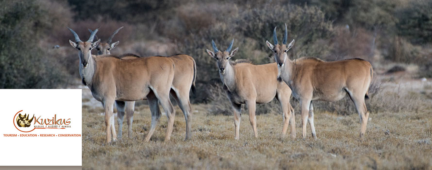
Our project is aimed at vegetation monitoring of the Kuzikus wildlife reserve in the Kalahari region in Namibia, Africa. Here we propose to develop deep learning models to predict the images of the vegetation cover over the reserve based on past satellite images.
The vegetation cover of the reserve changes every year based on several factors such as rainfall, and other natural conditions. The density of the vegetation is also hugely affected by the grazing patterns of the animals in the reserve.
As a result, if the vegetation in a particular area becomes sparse, the animals might lack necessary food and may die out. Our project aimed to prevent overgrazing and help the reserve to plan animal movement into areas of high vegetation density in advance.
Methods
Extraction of Satellite Data
We used the Google Earth Engine API which is a library that extracts archived NASA satellite images with all its spectral bands and metadata. Google Earth Engine is a geospatial processing service which provides python and Javascript API facilitates processing and downloading satellite images. The satellite images are archived in Google cloud storage and can be accessed in real time through the API.
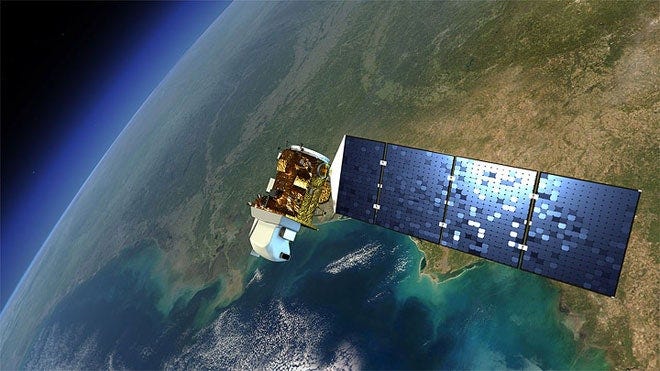
We selected LANDSAT-8 satellite images over other satellite images because it had multiple spectral bands which would be useful to detect vegetation cover, it had a reasonable spectral resolution of 30 meters and the most important factor — it provided the largest time series dataset which is required to make efficient predictions.
Analysing Satellite Imagery
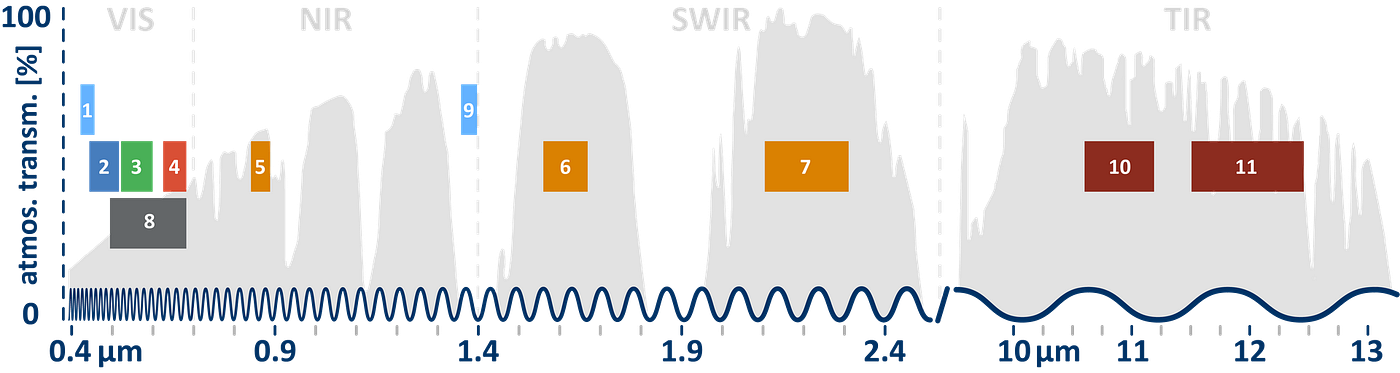
The information about the vegetation cover was extracted from the images of the area of interest. We used NASA’s LANDSAT-8 high resolution images of the earth, as the basic dataset for our analysis. We downloaded these images through the repositories from the NASA website for the satellite. The dataset consisted of 11 spectral bands with resolutions of 15m, 30m and 100m.
These images were Bottom of Atmosphere (BOA) and were atmospherically corrected. The metadata also provided coordinates for the exact location of the images captured. Upon visualization of this data using the Rasterio library, we noticed that the following spectral bands were available in the satellite data:
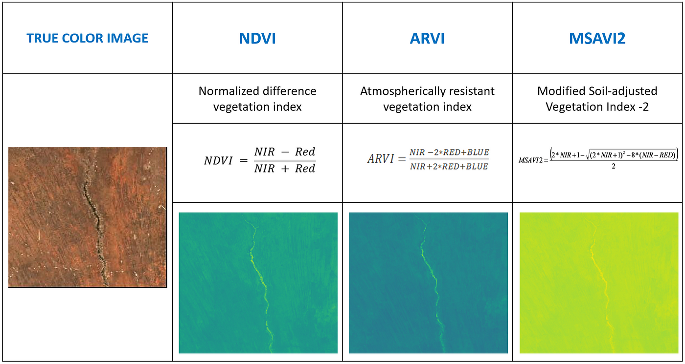
Various vegetation indices are frequently used to extract useful information such as vegetation density from the satellite imagery. Of these, we selected the following vegetation indices for our analysis:
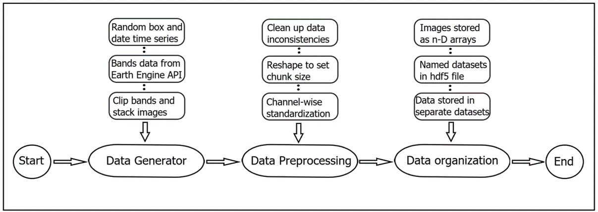
Dataset Creation
Once we had the API to extract the images, we had to create a time series dataset which would be used in the ML pipeline. This process was not trivial as the satellite images span more than 10000 square kilometers and usually the image data size would be more than 1 GB for a single timestamp. Thus, we needed an efficient way to process the images into required size to feed it into the ML pipeline.
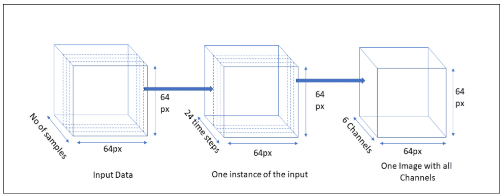
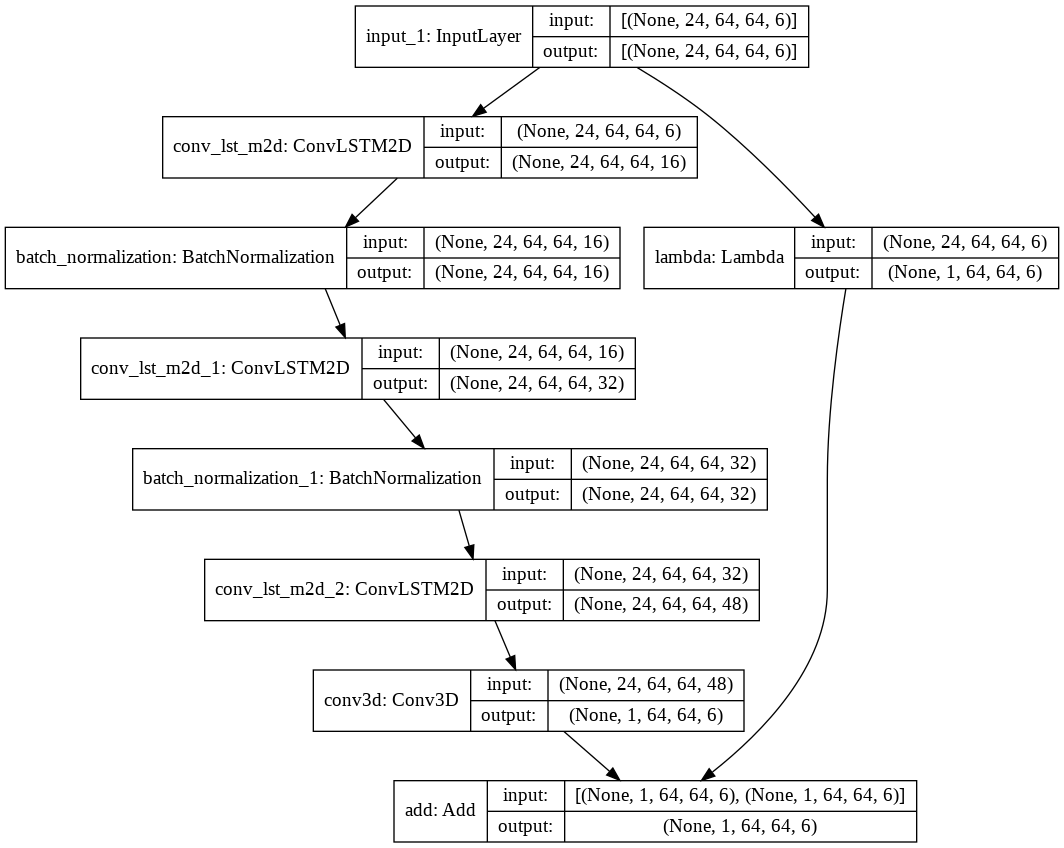
We decided to create a time series of images in which each instance has 24 images of the last 4 years with a 2 months interval. This instance of input data would be used to predict images six months into the future. For every instance we selected 6 images which consisted of 3 spectral bands — red, blue and green and 3 vegetation indices — NDVI, ARVI and MSAVI2. Thus, the input data would have the following dimensions: number_of_instances x image_height x image_width x timesteps x number_of_channels (n x 64 x 64 x 24 x 6).
Similarly, the ground truth data would have dimension: number_of_instances x image_height x image_width x timesteps x number_of_channels (n x 64 x 64 x 1 x 6). The time step would be 1 as there is a single image which is six months in the future from the instance timestamp.
To make input data more unbiased, we decided to extract random patches from the kuzikus reserve of 64 x 64 pixels in size. These image patches were about 1.5 sq km in area. For every data instance in the dataset, we generated 24 temporal images which spanned across 4 years with an interval of 2 months for the input data and 6 months into the future for the ground truth dataset.
Invariantly, the dataset created through this process was huge in size. Initially, we stored the dataset in the .mat file. But, this file format had file size restrictions. We switched to the HDF5 format (Hierarchical Data Format version 5) which is an open source file format that supports large, complex, heterogeneous data.
The HDF5 file format was more flexible and had no size restrictions unlike the .mat file. Further, to reduce the size of the dataset without compromising the quality of the data, we converted the dataset from floating point 64 precision to floating point 32 precision. This reduced the size of the data to half, as a result improving computation efficiency of the models.
Machine Learning Pipeline
After pre-processing and generating the time series dataset, our task is reduced to predict an image in the future given past images of the last 4 years. The image prediction task is not trivial and requires high computation and storage capacity to process the images. We implemented network models that Google Colab could handle.
Initial Architecture Plan
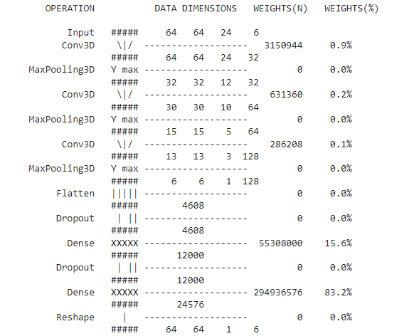
Initially, we designed two basic architectures — 3D CNN and ConvLSTM. In the 3D CNN architecture, we used 3D convolutions in the initial layers and dense networks in the final layers of the architecture. For the final layer, we transformed the flatten dense network into our required 3D ground truth dimension. This was the simple implementation with MSE loss.
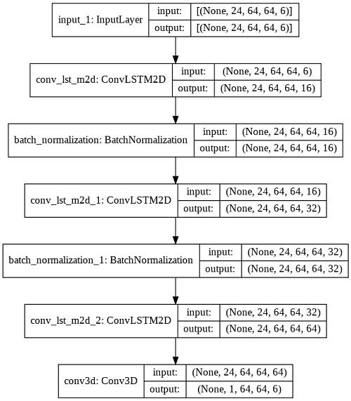
In our other architecture, we used ConvLSTM which is a variant of LSTM that uses convolution operation instead of normal matrix multiplication. This architecture is used to find temporal and spatial correlation. This model was also trained with the MSE loss. Both the models failed to learn and predicted images with multiple artifacts. ConvLSTM was better in a few cases but it required higher computation power to train the network.
Learnings from the Initial Architecture
We learned that these architectures failed because the network was not complex enough to predict the images. Also, we had to design a custom loss function to evaluate two images. We cannot use regular loss functions such as L1 or L2 as they do not accurately depict the similarity between images.
We implemented a loss function that is a weighted sum of L1, L2 and SSIM loss. The Structural Similarity Index (SSIM) is a metric that measures the similarity between two given images. The score ranges from 0 to 1, 1 being the highest similarity score. Keras Library provides a function to calculate SSIM loss.
def custom_loss(y_true,y_pred):
N = 1/(32*64*64*6)
l1_loss = N*tf.reduce_sum(tf.abs(tf.math.subtract(y_true,y_pred)))
l2_loss = N*tf.reduce_sum(tf.math.squared_difference(y_true,y_pred))
ssim_loss = (1-tf.reduce_mean(tf.image.ssim(y_true,y_pred,max_val=37)))
total_loss= 0.5*ssim_loss + 0.3*l1_loss + 0.2*l2_loss
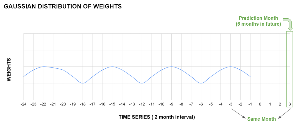
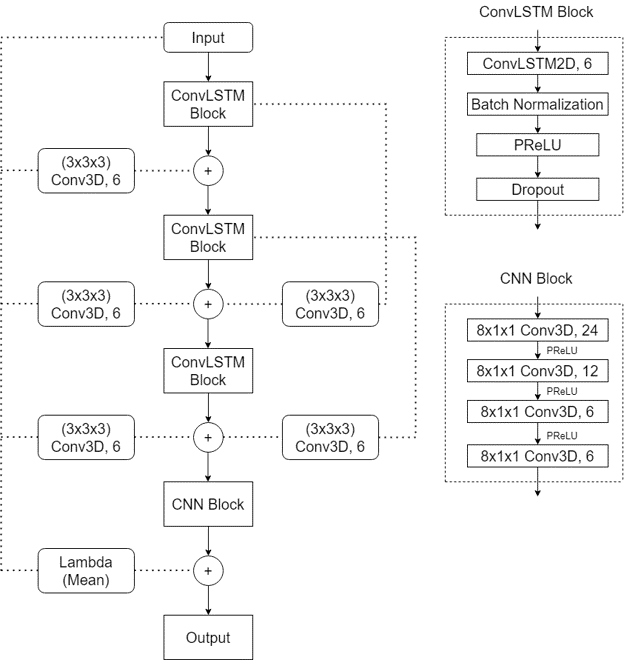
return total_lossFurther, we realized that the deep network would perform better with skip connections. We implemented skip connection that added the weighted mean of the 24 past images to the final layer of the architecture. The reasoning behind this skip connection function was that the image to be predicted in the future has certain factors such as water bodies, hills, big trees which remain constant with the past images of the same patch.
Also, while calculating the mean we weighted the images based on the seasonal similarities between them. For example, images predicted in the month of September 2021, the past images of September 2020, 2019 and so on were weighted more than the other images.
3D CNN & ConvLSTM with Skip Connections
The initial architectures were predicting results which had high losses and were deemed insufficient for our problem. We then implemented the above learnings — custom loss function and skip connections to the existing 3D CNN and ConvLSTM architectures.
With these implementations we see that the prediction had improved from the initial architectures but still lagged behind while considering accuracy of the result.
We observed that a single skip connection showed considerable improvement in result. To further investigate the scope of using skip connections, we implemented multiple intermediate skip connections in the architecture. As this model performed the best among all the models created so far, we performed hyperparameter tuning using Keras tuner. We tuned the following parameter: a) Filter size, b) Kernel size, c) Dropout rate, d) Learning rate and e) Type of Pooling
Result
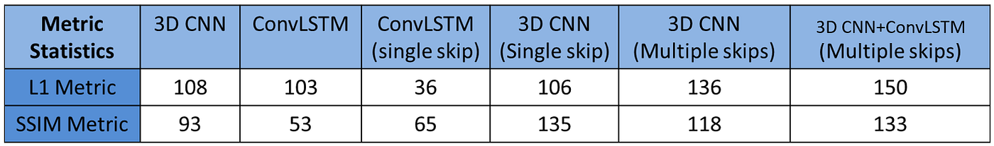
The model was evaluated against the labels on a set of 205 images and 133 of the predictions had an SSIM score greater than 0.8 SSIM and 150 of them had and L1 error below 0.4. A table showing the number of images satisfying this threshold is shown below for all the models tested.
Similarly, the L1 and SSIM metric of the predicted NDVI channel for the test input set.

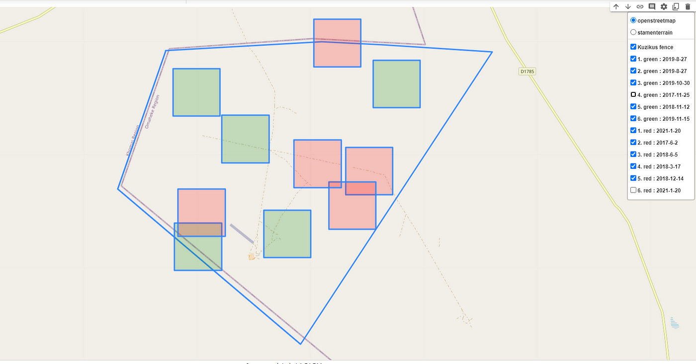
Finally, to visualize and geotag the region where the prediction was made an interactive map was created with the help of the Folium library by also including the coordinates data into the dataset. The image below highlights the regions where the predictions yield the highest and lowest SSIM scores with color codes and also labels them with the dates the prediction was made.
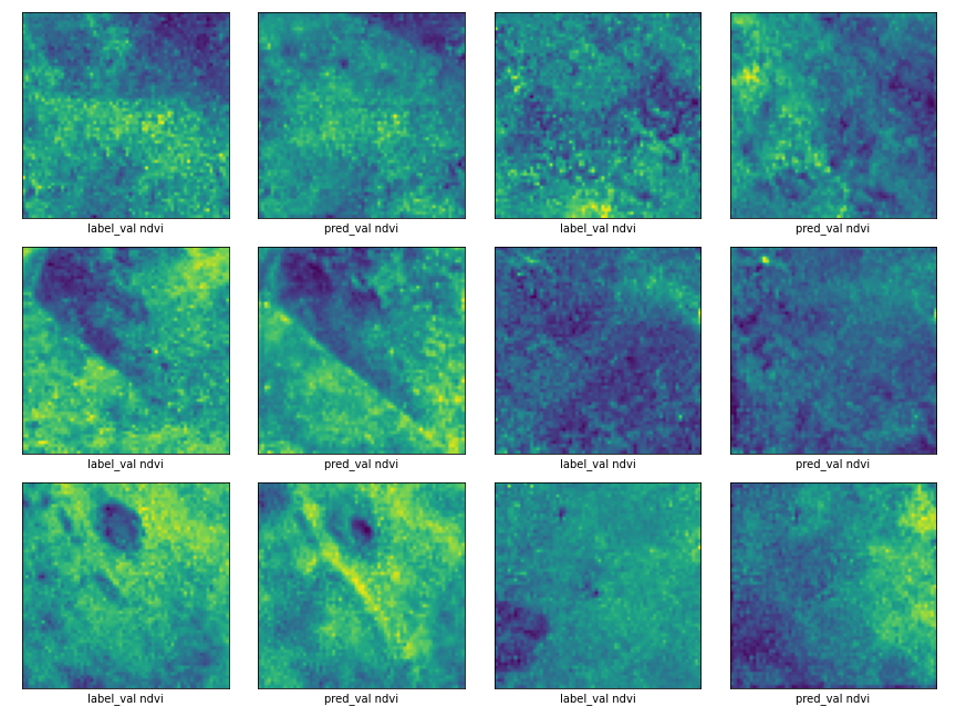
The prediction results for the NDVI channel are shown below for 6 samples. The label_val denotes the test set and pred_val denotes the prediction by the model.
Roadblocks in our project journey
During our project phase we faced certain issues while building the model. One of the problems we had was regarding the available spectral resolution of the satellite images. Predicting accurate vegetation density requires high resolution images but due to the limitation of the freely available satellite data we had to build our model using the best possible option.
Another issue that we faced throughout our model training phase was the lack of computational power. This was because our input data contains both spatial and temporal data instances and the size of the input data was considerably large. To train the model with such high dimensional data, a bigger dataset would aid in better model training, which might yield better results.
Conclusion
We observed that the problem we had was unique wherein we had to predict the vegetation in the Kuzikus reserve in the future by using the satellite image data from the past. To achieve this task we had to use a non-conventional approach wherein we had to find a temporal and spatial correlation between the data. The traditional ML models such as CNN and LSTM focused either on temporal or spatial correlation so, we developed an architecture that would learn and predict images based on both the dimensions.
We developed a 3D CNN + ConvLSTM with skip connections type architecture that proved to be much better than the traditional architectures. The results predicted by this model had a much better accuracy than the previous models and this could be a very useful insight to predict the vegetation in the reserve in the future.
Future Improvements
To achieve better accuracy we could train the model with a larger dataset. The quality of the input can be enhanced by using high spectral resolution images. Also, use of higher computational power to train deeper networks would result in significant improvements.