Detection of animals in drone images to support wildlife conservation in Namibia

Introduction

In recent years, Artificial Intelligence and Computer Vision algorithms have been developing rapidly due to the increase in computing power and its availability. These algorithms can be applied in a large variety of areas such as the detection of animals within landscape images. Wild Intelligence Lab is a non-profit organisation which aims to quantify wildlife reserves with the help of novel Computer Vision algorithms.

In association with the Kuzikus Wildlife Reserve in Namibia, many georeferenced orthomosaics of specific natural reserves are captured with drones and available for use by the Wild Intelligence Lab. These high-resolution drone images provide essential data for training a neural network, which can be used to detect and count the wildlife population, saving time and money.

Our TechLabs project aims to count the number of wildlife present in images collected from the Mahango area in the Bwabwata National Park with the help of convolutional neural networks for object detection. This article will describe the chosen methodology and present our findings.

Figure 1. Semi-aquatic wildlife in Mahango core are of Bwabwata National Park.

Methods

Data preparation

As mentioned in the introduction, the dataset consists of numerous orthomosaics. Each orthomosaic combines smaller images called orthophotos and gives a relatively clear view of a wide area. For this project, there are about two thousands such orthomosaics with a resolution of 2048×2048 pixels.

Since all orthomosaics are raw data and don’t contain information about the animals present in them, we need to label the images for model training. As there is a massive amount of images and some of them are blurry or contain a large blank area, we decided to remove such images from consideration for the labeling process using two functions.

We applied the variance of Laplacian method to characterize how blurry a picture is. If the variance fell below a predetermined threshold (800), the image was marked as blurry and discarded. We tried different threshold values starting with a much higher value than 800 and then manually checked if the sorted images were actually blurry or not. Then, the threshold was decreased slowly until only non-usable images were sorted as blurry.

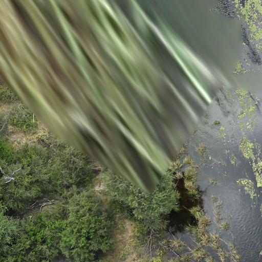Figure 2. Example of a blurry image.

OpenCV-Python was used for detecting the blank area of a picture. We converted color images to grayscale using cv2.cvColor() method. Since all blank areas were completely black, the percentage value of black pixels refers to the darkness in a picture. We set 35% as the threshold for the reason that some pictures with small dark areas can contain animals as well. The image was only removed if the calculated rate exceeded 35%.

All orthomosaics were passed through the above functions and only the usable images were considered for the manual data annotation.

Figure 3. Example of blank image.

After data cleaning, we selected VOTT, an open source annotating app, as the tool used for annotation. Animals can be labeled with bounding boxes. Based on the local ecosystem conditions, we considered two ways to label wildlife in the images from Mahango. Aside from having land regions, Mahango contains many rivers and lakes. We observed that the images contain both animals which were found on land or within the waterways.

Since the animals appear differently when in the water or on land, we decided to use two class labels: “Land animal” and “Water animal”. Note that e.g. a crocodile can be labeled as both classes in different images, depending on whether it is within the water or on land. We thought that using two different labels for land and water animals would simplify the object detection, but when we were training the first models, the performance was bad. As a consequence, for later training we decided to merge the two labels into one — “Animal”.

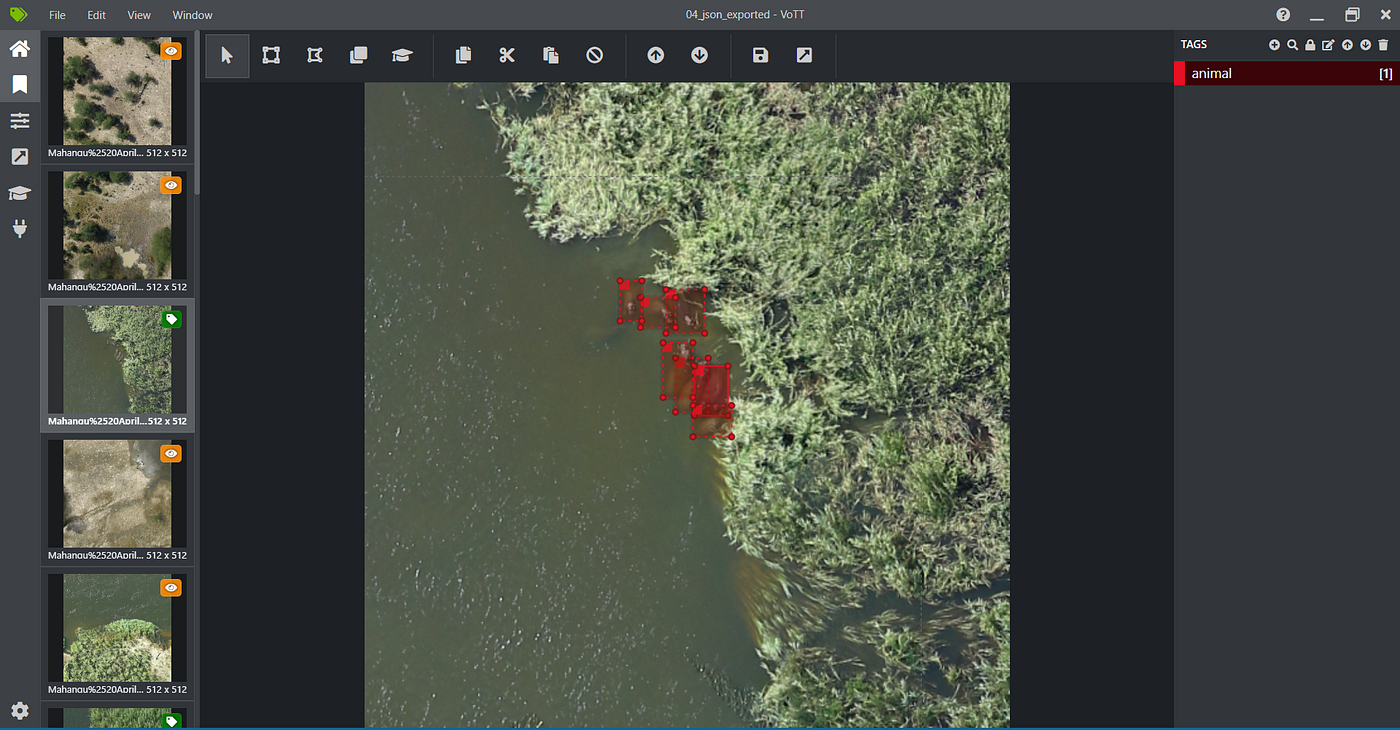
Figure 4. Example of a labeled image.

177 images in total were labelled which contained 607 animals and an additional 177 negative images (without animals) were added as input. In total 354 images were split into Training, Validation and Test set at a 70:20:10 ratio (Training — 248, Validation — 71, Test — 35 images). These pictures were exported as csv files by VOTT, which contained the bounding boxes with four columns (xmin, ymin, xmax, ymax). This format complied with the requirements of most CNN object detectors for model training.

Object Detection

For object detection in images, new neural network architectures are continuously being developed but are always extensions of convolutional neural networks (CNNs). CNNs are deep networks with several layers and extract the features in the images that are used for certain predictions. Within an object classification framework, CNNs learn to extract the important features that can distinguish objects from background in the images (figure 5).

This is done by sequentially detecting low-level to higher-level features: the first layer usually learns to detect edges, the second combines edges to detect shapes and structures, whereas the last layers can detect entire objects. The last step in the object detection CNN is a regression on the features of the last layer for classification.

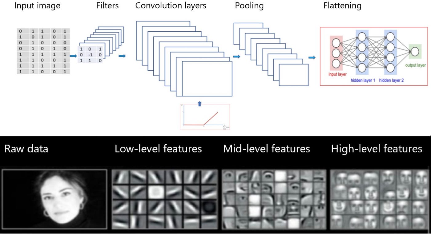
Figure 5. CNN architecture. Adapted from NVIDIA and towardsdatascience.com

When objects are not centred but can be anywhere in the image, such as in our data, the model should both classify objects and locate them, or give the ´bounding boxes´ (x- and y-coordinates, height and width of the object). Therefore, and because multiple objects of different sizes can be present, it is not possible to feed the entire image directly into a CNN for classification. Instead, smaller zones of the image are selected to perform classification on separately (target region selection).

This can be done by simply using sliding windows of varying sizes or by a more complex selection method. To summarise, object detection algorithms for images without centred objects usually consist of three steps: target region selection, feature extraction and regression for classification/bounding box prediction.

Currently there are two main object detection methods available: two-stage detectors (e.g. faster R-CNN) and one-shot detectors (YOLO, SSD; see figure 6). Two-stage detectors first perform target region selection with an additional region proposal network that selects regions on a feature map instead of on raw pixels, which is much faster than sliding windows. Then, objects are detected in only the selected regions by an additional network.

By contrast, one-shot detectors detect all objects within an image in a single forward-pass of the network: the image is divided into a grid and in each grid cell the class and location of objects -when present- are predicted along with a confidence. Simultaneously multiple anchor boxes with predefined sizes are assigned to each grid cell, which are then matched with the highest-confidence detected objects. Finally the anchor boxes with the biggest overlap are selected as bounding boxes for the detected objects.

One-shot detectors such as YOLO are very fast and therefore currently one of the most popular architectures used for real-time object detection in videos. Since our project does not do real-time detection and the trade-off is decreased accuracy, we decided to start with faster R-CNN, which is one of the most popular two-stage detectors.

Compared to the one-shot detectors, this model also fits our dataset better: accuracy is higher for the detection of small objects and objects close to each other, for generalisation to different aspect ratios, and for smaller datasets. In addition, we tried a few other models to be able to compare the results.

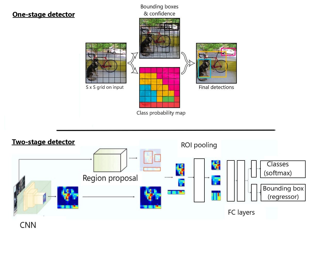
Figure 6. One-stage detector (above) and two-shot detector (below) architecture. Adapted from pyimagesearch.com and datadriveninvestor.com.

Instead of training a model from scratch, we decided to use transfer learning. Transfer learning is the approach of using a model that was pre-trained on a bigger dataset as the starting point, and only needs fine-tuning to suit the new task. Generally only the last layer or last few layers are re-trained on the new dataset, which results in a more accurate model.

For object detection transfer learning, two big datasets exist that are freely available: ImageNet and COCO. ImageNet consists of 1.4 million annotated images with one centred object per image grouped into 3000 classes, while COCO consists of 200 thousand annotated images with 1.5 million objects depicted in their context and grouped into 90 classes.

We decided to use models that are pre-trained on COCO images as these better resemble our dataset: several objects can be present in one image and they are usually not centred. Also, our images do not contain a high number of different classes.

As Tensorflow has various models build-in that are pre-trained on the COCO dataset, we chose to use the following different models from the TF2 Model Zoo: faster R-CNN Resnet152, CenterNet Resnet101, and EfficientDet D0.

Object Detection Metrics

For the comparison of the above selected object detection models, we needed appropriate metrics to evaluate and compare the models. Object detection metrics serve as a measure to assess how well the model performs on an object detection task. In computer vision, mean Average Precision (mAP) is a popular evaluation metric used for object detection (i.e. localization and classification). Let us understand this metric.

In a simple classification task, it is straightforward to identify correct predictions from incorrect ones based on the probability of the object class. However, the object detector localizes the object further with a bounding box associated with its corresponding confidence score to report with which certainty the bounding box of the object class was detected.

Therefore, to determine how many objects were detected correctly and how many false positives were generated, we use the Intersection over Union (IoU) metric (figure 7). IoU measures the overlap between the ground truth box and the predicted box over their union. The IoU score ranges from 0 to 1; the closer the two boxes, the higher the IoU score.

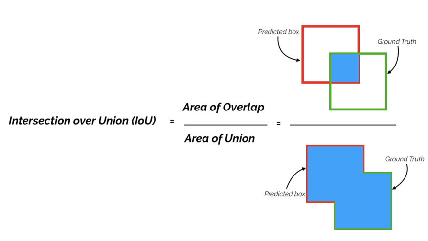
Figure 7. Intersection over Union.

The predictions are classified into True Positives (TP), False Negatives (FN), and False Positives (FP). A prediction is classified as TP if the IoU is greater than an IoU threshold and class prediction is correct. A prediction is classified as FP if the IoU is less than an IoU threshold or if it is a duplicate bounding box. A prediction is classified as FN if there is no detection or the IoU is greater than an IoU threshold but class prediction is incorrect.

Precision, Recall and the Precision-Recall curve

Precision is the probability of the predicted bounding boxes matching actual ground truth boxes, also referred to as the positive predictive value (figure 8). Recall is the true positive rate, also referred to as sensitivity, which measures the probability of ground truth objects being correctly detected (figure 9).

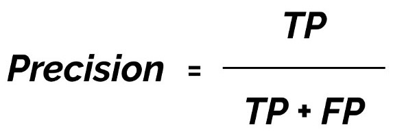
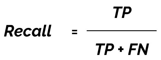
Figure 8. Precision formula.

The object detector predicts bounding boxes, each associated with a confidence score. By changing the confidence threshold, we get different TPs, FNs, FPs and thereby different precision and recall values. For a particular class and IoU threshold, we plot the precision and recall values while varying the confidence threshold to get a precision-recall curve (figure 10).

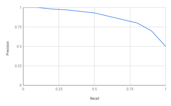
Figure 10. Precision-recall curve.

Average Precision (AP) and Mean Average Precision (mAP)

Average precision (AP) serves as a measure to evaluate the performance of object detectors. AP is a single number metric that encapsulates both precision and recall and summarizes the Precision-Recall curve by averaging precision across recall values from 0 to 1.

It is effectively the area under the precision-recall curve. Mean average precision (mAP) is calculated by taking the average of AP over all classes and/or multiple IoU thresholds. The COCO Object Detection Challenge evaluates detection using 12 metrics. One of the metrics is mAP (interchangeably referred to in the competition as AP) which is the principal metric for evaluation in the competition, where AP is averaged over all 10 thresholds and all 80 COCO dataset categories.

Hence, a higher AP score according to the COCO evaluation protocol indicates that detected objects are better localized by the bounding boxes. We have used this metric for the comparison of performance on our dataset of the different object detection models, which we selected from the TensorFlow 2 Object Detection Model Zoo.

Results

This part demonstrates and compares the final results of three different object detection models using mAP as the benchmark.

For the model training we considered three data augmentation options: “without augmentation”, “with 8 augmentation methods” (horizontal_flip, vertical_flip, rotation90, crop_image, hue, contrast, saturation, brightness), and “with 3 augmentation methods” (horizontal_flip, vertical_flip, rotation90). The best mAP turns out to be different under these three situations.

We decided to train all models using the augmentation option with 8 functions, so that their performance can be directly compared. See the results table (figure 11) for these mAP values. The “AG Graph” column indicates the development of the mAP value during training of the three models and “Best AP” column is the highest value that the model can achieve.

Faster R-CNN ResNet152

Faster R-CNN without augmentation exhibited a mAP value of 0.075. It increased to 0.13 after the addition of the 8 augmentation methods. This demonstrates that Faster R-CNN with augmentation performs better as it makes the model more robust to different kinds of input. The total training loss decreased for both models as we continued training for 25k epochs.

However, the total validation loss seemed to increase slowly after 11k epochs. This shows that the model starts to overfit the data after 11k epochs. Hence in case of Faster R-CNN, the model should be trained for around 11k epochs.

CenterNet Resnet101

The mAP for CenterNet Resnet101 increased dramatically from 0 to 10k epochs, then fluctuated and peaked at 42k epochs with 0.1732. Without data augmentation functions, this model had a lower mAP value of 0.0917. Again training the model with augmentation outperformed training without augmentation. The total loss dropped from 18 to approximately 2 at 10k epochs and stayed quite constant thereafter. CenterNet Resnet achieves a satisfactory result since it has a relatively higher mAP.

EfficientDet D0

The model Efficientdet D0, when trained without augmentation has a constant mAP of 0. While using the data augmentation functions, the highest mAP value achieved was 0.093. The mAP value for the version of the model with data augmentation was not constant like in the case without any augmentation. Instead it increased overall from 0 at 0 epochs to 0.093 at 50k epochs with numerous fluctuations in between.

The model was trained for 50k epochs, but the total training loss seemed to be unchanging after 4k epochs for the version with data augmentation. While manually testing the trained model on a small number of random images, animals could not be successfully detected.

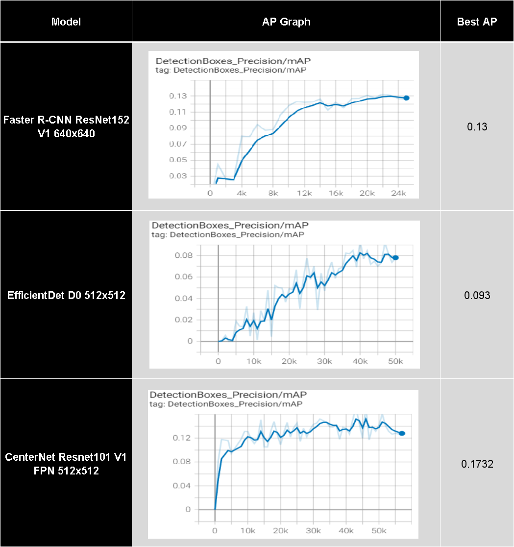
Figure 11. The table compares the mAP values of the three models using the mAP graphs and best mAP value.

Overview

Comparing the three different models, as shown in the table above, we see that the CenterNet ResNet model has the best relative mAP. We can further note that this mAP is achieved while using the 8 chosen data augmentation functions. Upon testing this model on a set of 35 images, it was observed that the model could successfully detect a significant number of animals. It is important to note, that the confidence threshold used for this testing was 3%.

This threshold was chosen in order to see the performance of more bounding boxes. Using lower confidence thresholds led to some correct and incorrect detections. Several examples of the output of the model when applied to images from the test set are shown in Figure 12.

Figure 12. Examples of the output of the model when applied to images from the test set.

The next best result was achieved using the Faster R-CNN model, with the second highest mAP of 0.13. The last model, namely EfficientDet had a low mAP value of 0.093. This suggests this model either does not work well with the small volume of training data, or for the goal of the project. The model possibly need modifications and more labelled training data in order to obtain a better outcome.

The dataset used for training contained a small number of labelled animals, which were all of various species, in a large variety of environments, resulting in few examples of each specific species in specific environments. This is probably part of the reason for the poor performance and confidence of the models, and training one of the better performing models with a larger labelled dataset would be able to further improve the predictions and confidence.

Figure 13 shows examples of output images where some animals in the images were not detected by the model.

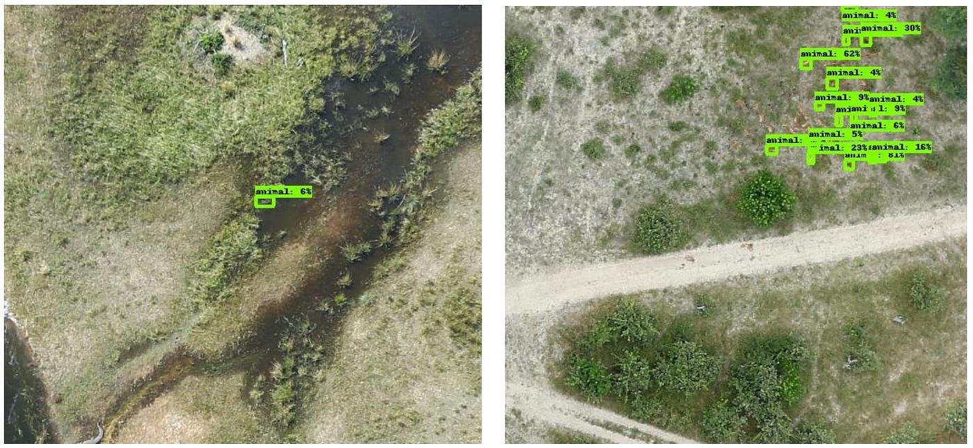
Figure 13. Example of an output where a few animals were not detected.

Conclusion

In conclusion, we found that automated detection of semi-aquatic wildlife could be achieved using Machine Learning models with varying degrees of accuracy.

It is widely known that under normal circumstances wildlife numbers do not change rapidly. Due to these changes being small and gradual, regular counts are needed to detect them. The dataset used includes images of not only land but also of water and marsh land regions in the Mahango core area in Bwabwata National Park. Because the method used in this project to count animals does not depend on ground access to the wildlife area, these counts can be carried out more frequently in the future.

Therefore, the insights gained during this project could allow conservation managers at the Mahango wildlife reserve to use drone-acquired imageryand machine learning algorithms more accurately and efficiently to gather valuable information about vulnerable populations and ecosystems, which can be critical for their conservation. While the project provides a useful result, we should also note that bigger volumes of training data are needed to obtain a more reliable detector.

Sources and References

Authors

Bharath M
Evelina
Hanna van den Munkhof
Hansika Zaveri
Lea Jaklen
Mansi Patil
Varum Chintapally
Yanyuan Lu

Do you have any comments, ideas or hints for this post?

Then contact us!