Introduction
Technology in wildlife conservation:
Technology has been evolving to new standards catering not only just human needs but also to protecting and conserving the living organisms in this universe. The main concern is to preserve the flora and fauna of the wildlife so that future generations of wildlife and even humans can enjoy it. Wildlife conservation is one such field where the use of technology has been gradually increasing and reaching new limits day by day. Thanks to the advancements in cameras and Machine learning algorithms which helped scientists and activists to analyze and act upon the dynamics of wildlife conservation more accurately and effectively.
The Earth has several species of living beings on it and it is very fascinating to see all these living organisms play an important role in keeping the food chain intact and hence allowing all the living things to survive and evolve. So as supreme predators in this food chain it is our responsibility to make sure protect the wild in nature. Methods of wildlife conservation must accommodate the emerging technologies. Fortunately, several countries and their esteemed institutes along with different organizations are coming forward to integrate technology and conservation methods.
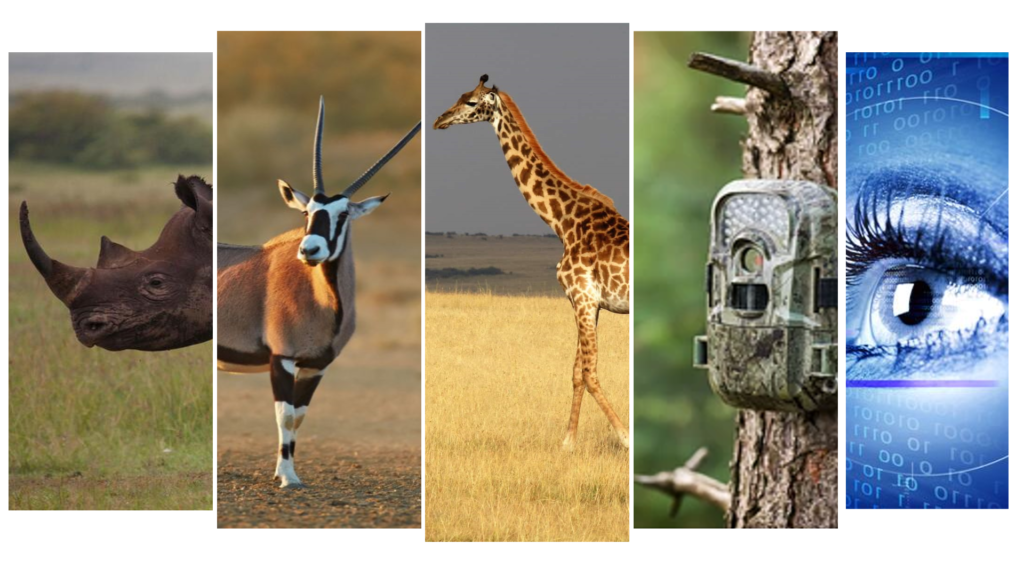
Fig. 1: Image source [https://www.shutterstock.com]
Wild Intelligence Labs (WIL)
At Wild Intelligence Labs, Scientists, Engineers, and nature conservationists share a common goal to integrate technology and conventional conservation techniques and produce sustainable solutions. WIL in partnership with Dr.Friedrich Reinhard from the Kuzikus Wildlife and Nature Reserve (Namibia) is testing these developments for implementation in the nature reserve.
Kuzikus provides the perfect environment to test and develop such technology and one such application is being developed by Wild Intelligence Labs. The main objective of this project is to train a model that continuously counts the number of animals in images provided by a network of Nvidia Jetson-based Edge devices in Namibia to gain insights into animal behavior and monitor them. The wildlife reserve at Kuzikus (Namibia) is known for several species of wild and is divided into 13 categories for this project. Several state-of-the-art Object Detection models will be implemented on the data set to classify and count the different animals in each image at real-time. These trained models will be evaluated and the best performing will be selected and integrated into Nvidia Jetson Nano.
Method
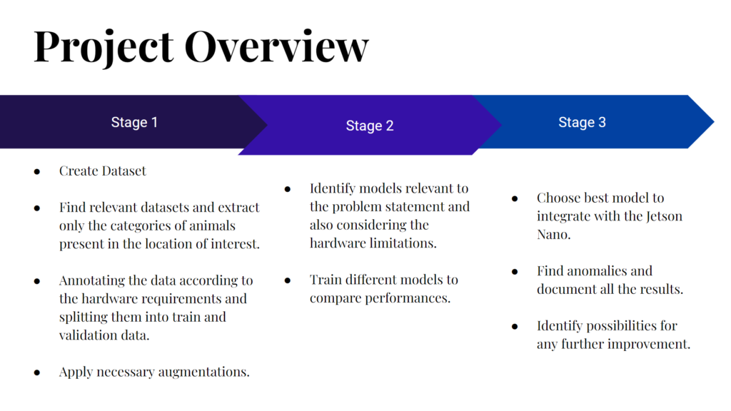
Fig. 2: Project Overview
Stage 1: Dataset Creation
WIL provided us with a dataset of around 1.000 images. As this is not large enough to apply Transfer Learning we needed to expand the dataset.
To do this, we explored different freely available Datasets and collected all images containing the needed species. In addition to the animal images, we also collected a small sample of human and car images. This was done because the flora and fauna of any natural reserve are constantly posed by the threat of poachers and their illegal activities. This way the models shall also be able to detect possible poachers.
After collecting the dataset we needed to annotate around 12k images because the datasets were mostly only annotated with labels and not bounding boxes. This was done using the CVAT annotation tool. It took several hours to manually annotate these 12k images using 2 point bounding box method. Later all these images and annotations were exported to different formats like YOLO and Pascal VOC as needed.
In the end, our dataset contained 14606 images with the following bounding box count for each species:
‚eland‘: 4057
‚giraffe‘: 2266
‚impala‘: 4061
‚jackal‘: 1122
‚kudu‘: 338
‚ostrich‘: 1891
‚rhino‘: 676
’springbok‘: 721
‚zebra‘: 4705
‚oryx‘: 482
‚car‘: 785
‚human‘: 756
‚other‘: 529
Several challenges were faced while annotating images. The most concerning were:
1. When there is a large number of animals occluded by each other animal. This was dealt by annotating the background animal assuming its full form.
2. There are certain instances where only less than 20 percent of the animal body is within the frame. Such cases were ignored. As our main goal is to work on a video stream. This problem wouldn’t be an issue as we can detect such animals in several previous frames.
3. There were other animals rarely identified in the image dataset which we have included under the label „other“.
4. Animals were sometimes occluded by large structures like bushes, trees, and rocks. We didn’t have several of such animals to annotate but to make our model robust to occlusions we have decided to annotate them as well and augment the data accordingly in the later phase of data preparation.
5. Several animals were in distinct poses and found in different weather conditions. There could be a high chance of overfitting because of the limited annotated data we had but we have managed to find suitable augmentations to deal with overfitting to some extent.
Augmentations
Augmentations are generally applied when there is a danger of overfitting or the model not being generalized based on the training data. Collecting more data may solve the problem in such cases but considering the time taken for annotating data, it is always better to apply augmentation techniques which saves a lot of time in the data preparation process.
Data Augmentation is a technique where we expand the dataset size artificially by modifying the existing data using techniques like Geometric transformations, Color space transformations, Kernel Filters, etc.
For this project, we have used our own data augmentation pipeline which can be used on any animal dataset in wildlife. The python library used for this project is Albumentations as they efficiently implement a large variety of image transformations which enhances the performance of deep convolutional neural networks. It is superior in performance, variety and also quite flexible in research and can easily be adapted to changes when compared to other available libraries.
The following augmentations were used,
A.Resize, A.Rotate, A.HorizontalFlip, A.RandomRain, A.RandomSunFlare, A.RandomShadow, A.RandomFog, A.ToGray, A.RGBShift, A.GaussNoise, A.MotionBlur, A.MedianBlur, A.Blur, A.ShiftScaleRotate, A.RandomBrightnessContrast, A.HueSaturationValue
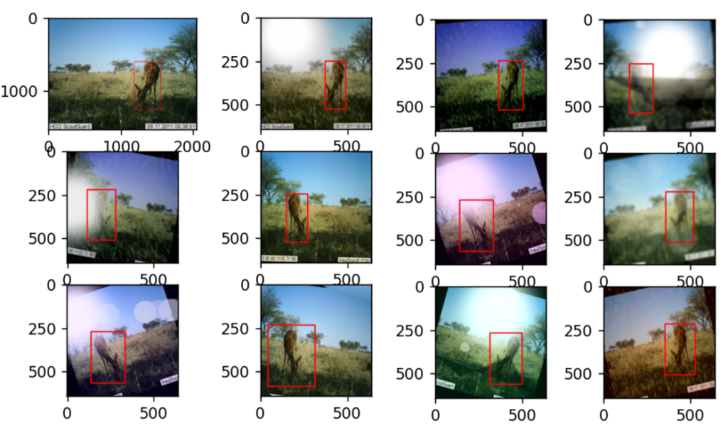
Fig. 3: Example of augmentations applied to an image
All these augmentations are chosen specifically to meet the various scenarios we can find an animal in wildlife. There could be several weather changes and lighting effects on the animal and also on the camera lens. Considering all these effects these augmentations are selected.
Stage 2: Model selection
In the past few years, the research in deep learning techniques has achieved several efficient models for object detection for various use cases be it in Defense, Agriculture, Medical, Environment, Food Processing, Robotics, etc. Several models have been detailed throughout these years of the development phase. Many of them are used specifically for certain user applications and one such application we have tried to explore in this project is object detection of animals in nature conservation areas where the main objective is to count the number of animals belonging to different species identified in a real-time setup. In order to accomplish real-time object detection given the hardware requirements of the Nvidia Jetson Nano, we decided to focus on two different models. Those models were chosen because of the performance graph of the Jetson Nano provided by Nvidia.
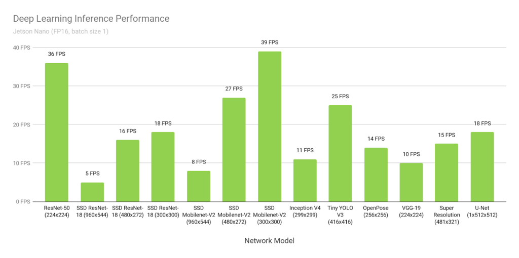
Fig. 4 : Deep Learning Inference Performance on Nvidia Jetson Nano
The first model family we decided to focus on are the YOLO models. YOLO which stands for “You Only Look Once” is a family of Convolutional Neural Networks that is a set of end-to-end deep learning models for efficient object recognition. Although the models‘ accuracy is not as high as that of heavier models, it still produces comparable accuracy and is very popular for real-time object detection because of its speed. There are currently different YOLO versions available. Here we will focus on the YOLOv5s, a heavier model promising better accuracy, and the YOLOv3-Tiny, a lighter model promising good inference speed with reduced accuracy.
We chose two different versions because we found different inference performances for the YOLOv5s model when running on the Jetson Nano, reaching from not suitable for real-time detection on the Jetson Nano to 15FPS. Because of this uncertainty, we chose the YOLOv3-Tiny as our backup model in case the YOLOv5s is too heavy for the Jetson Nano.
The YOLOv3 Tiny model is a simplified version of the YOLOv3 model because it has a smaller number of CNN layers and hence it doesn’t occupy large memory as a YOLOv3 model does. This also improves the detection speed and also reduces the hardware dependency. But thee is a trade between reduced accuracy and the above-mentioned advantages of using a tiny version of YOLOv3
The YOLOv5s model is the second smallest YOLOv5 model available. It promises higher accuracy and increased inference speed than previous YOLO versions. Only the Tiny versions of YOLOv3 and YOLOv4 have higher inference speed.
The other model family we focused on in our project are the SSD MobileNet models. It belongs to a class of lightweight deep convolutional neural networks that are much smaller and faster than many of the mainstream popular models. MobileNets are a class of low-powered low latency models that are mainly used for applications like classification and detection. So this model works well when there are limitations on the processing hardware. Because of their size, MobileNets are often considered great for mobile devices.
Stage 3: Applying the Best Model to Jetson Nano
In order to be able to apply the trained model onto the Jetson Nano we first needed to set up the environment for the Jetson Nano. Furthermore, we used TensorRT in order to improve the inference speed of our trained models.
Project Results
We were successful in training the YOLOv5s and YOLOv3-Tiny models, using PyTorch, obtaining quite good results with regard to our dataset.
In contrast to that we were not able to train the SSD MobileNet, using Tensorflow, due to some issues we faced which could not be resolved due to lack of time.
Applying the successfully trained models to the Jetson Nano also introduced some challenges. In the end we were able to apply the models to the Jetson Nano but then we were facing serious performance issues. We could not reproduce the promised 25FPS for the YOLOv3-Tiny model although using TensorRT in order to boost performance.
YOLOv5s and YOLOv3-Tiny

Image source: pytorch.org
Both models were trained for 186 epochs on our dataset using the PyTorch implementation provided by Ultralytics(https://github.com/ultralytics/yolov5). The results are quite good for both models. But, as expected, the YOLOv5s model was able to fit the dataset better due to the fact, that it is a heavier model compared to YOLOv3-Tiny.
YOLOv5s `Precision: ≈88%` `Recall: ≈84%` `mAP_0.5:0.95: ≈65%` `mAP_0.5: ≈88%`
YOLOv3-tiny `Precision: ≈81%` `Recall: ≈71%` `mAP_0.5:0.95: ≈48%` `mAP_0.5: ≈79%`
During training we used the SGD Optimizer with Momentum Method and a Learning Rate Scheduler.
The training was divided into different Runs. After each separate Run we adjusted some hyperparameters, but especially the starting point of the learning rate. During each Run the Learning Rate Scheduler linearly decreased the learning rate from the set starting point until nearly 0 when reaching the end of the Run.
At the end of training we encountered first signs of overfitting.
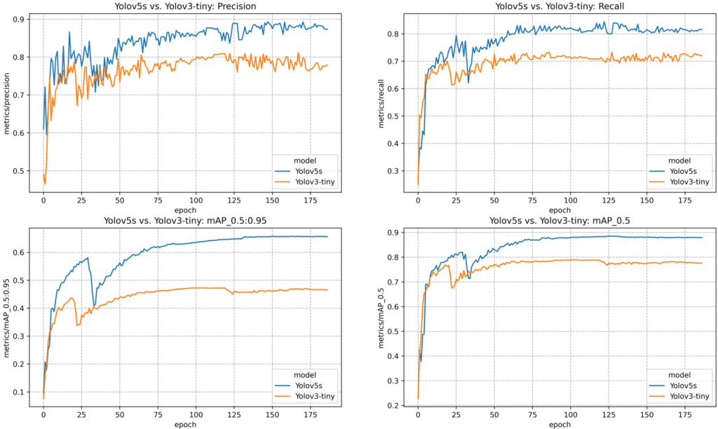
Fig. 5: YOLOv3-Tiny and YOLOv5s in Comparison
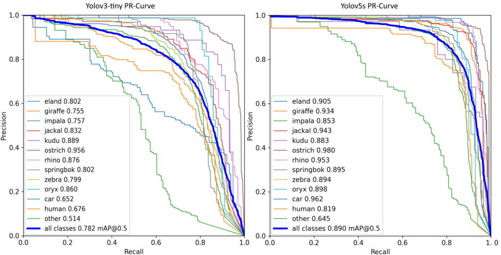
Fig. 6: PR-Curve of YOLOv3-Tiny and YOLOv5s in Comparison
The more the PR-Curve is bent to the top right corner, the better the model.
SSD MobileNet V1

Image source: tensorflow.org
The TensorFlow Object Detection API is an open-source framework built on top of TensorFlow that makes it easy to construct, train and deploy object detection models. It includes a collection of pre-trained models in their framework referred to as Model Zoo. A pre-trained version of SSD MobileNet V1 is available in their Model Zoo. So, we decided to use the API.
The following image represents the loss results while training SSD MobileNet during an epoch with a gradually decreasing learning rate. It was observed that there were some fluctuations in the loss functions, but overall the loss was gradually decreasing. These results are visualized using Tensorboard.
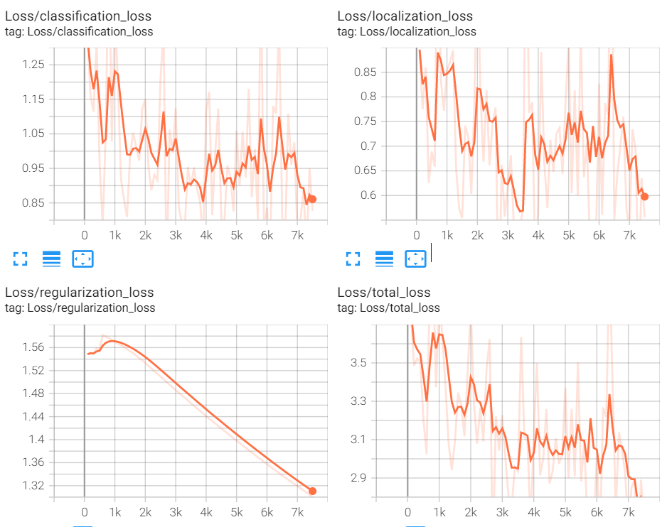
Fig. 7: Loss Curves for SSD MobileNet V1
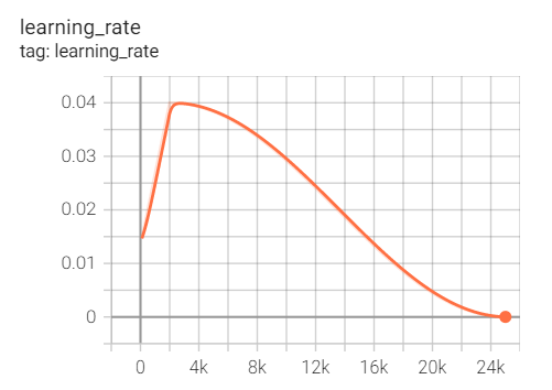
Fig. 8: Learning Rate Curve for SSD MobileNet
While working with the API we faced various challenges in the pre-processing phase and training phase.
The format of the data generated from CVAT is much different compared to the Pascal VOC format required for generating tfrecord files which is requirement of tensorFlow object detection API. As a result, various errors were encountered while the converting the annotations. e.g. In CVAT IDs of the classes start from 0 whereas in API 0 is reserved for background also in CVAT based on how bounding boxes are drawn order of dimensions of bounding boxes is defined but API needs the dimensions in a certain specific order. As all these errors were found during different steps of training, finding the cause of these errors and then writing python scripts for solving those was challenging.
Not a lot of information is available online about the model configuration files. Hence, it was quite difficult to understand how to tune hyperparameters, how to freeze the pre-trained layers, and ultimately how to improve the performance of the model.
Nvidia Jetson Nano
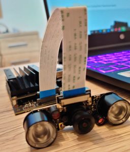
Fig. 9 : Nvidia Jetson Nano
When we got our hands on the Nvidia Jetson Nano the first thing we did was to set up the Jetpack image which contains the Jetson Linux and a handful of other developer tools such as TensorRT and CUDA. Then we proceeded with the installation of all the required dependencies and packages and this is where we started facing some obstacles of missing modules or versions mismatch. All of that led to a lot of time spent troubleshooting and fixing the problems.
In the end, we were able to apply the YOLO models to the Jetson Nano. We will provide the WIL with the Step-by-Step installation guide because small deviations from this can cause serious problems often resulting in the need for reinstalling the JetPack OS.
After successfully initializing the Jetson Nano with all needed packages we applied the YOLO models using TensorRT in order to do a benchmark regarding the inference speed. Sadly, we were not able to reproduce the promised performances stated by Nvidia. While the YOLOv3-Tiny model required around 500ms for each image to be inferred, the YOLOv5s inference speed fluctuated between 900ms and 100ms per image.
Due to lack of time, we were not able to investigate this problem any further, leaving some work for future TechLabs students.
Conclusion
All in all our project was a tough challenge in itself and a lot of new skills were acquired along the way. We want to thank Techlabs Aachen e.V., Wild Intelligence Labs and our Mentor for this opportunity and their support.
The trained models will be provided separately with additional evaluation materials and a step-by-step installation guide for the Nvidia Jetson Nano.
Although we were not able to apply the models to the Jetson Nano while meeting the real-time inference speed requirement we still managed to train the models which can be applied to Camera Traps in the future.
Further Improvement
– The Dataset can be expended as the YOLO models showed signs of overfitting. It is also recommended to look at the already annotated images as we noticed some annotation inconsistencies inside the collected datasets.
– The YOLO and SSD models can be further fine-tuned through training them for even more epochs while optimizing the hyperparameters.
– There is also still a lot of work to do in order to reach the promised performances when applying the models to the Jetson Nano.


