Shadow Detection for Wildlife Management (Part II)

Introduction

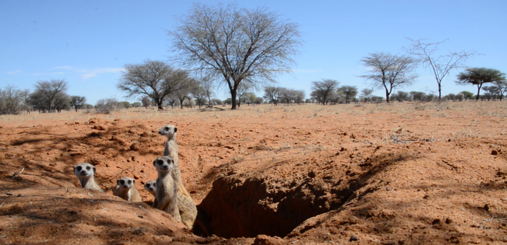
As ecosystems are increasingly threatened by rising land use pressure due to human population growth and climate change, effective wildlife management becomes vital in preserving and protecting ecosystems. Traditional methods, such as manual counting of different animal breeds or the recognition of landscape features in bounded areas, are often too complex or expensive to implement. In cooperation with the Kuzikus Wildlife Reserve in Namibia, the non-profit organization Wild Intelligence Lab aims to address these issues. Through the use of innovative technologies such as machine learning algorithms, WIL devotes itself to make a lasting impact on the conservation of ecosystems.

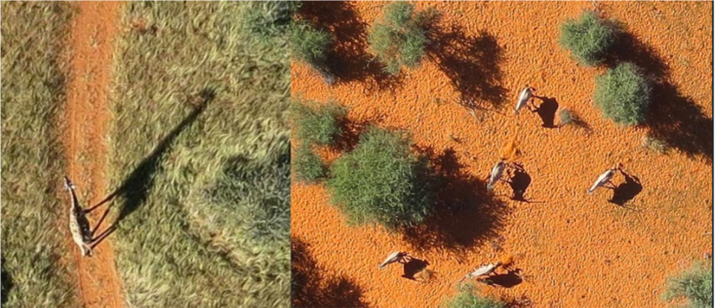
So far, counting and detection of different species and landscape features from the ground is a long and time-consuming process that can hardly provide a good coverage of landscape. Earlier, attempts have been made to record the landscape with the help of a camera from a helicopter, but this posed a problem to the animals living in the wildlife reserve as they tend to get agitated by the noise and the shadow cast by the helicopter. In order to address these issues, unmanned aerial vehicles (UAVs) or satellites are used to capture high resolution images of the wildlife reserve along with the geo-referencing information.

Taking this problem into account, our TechLabs project starts to contribute an important part to wildlife conservation by using emerging technologies. The following paragraphs describe the developments up until today and are intended for readers of all backgrounds. We hope to give you a detailed insight into the intersection of Wildlife Conservation and Technology and encourage you to contact us in case of any questions.

Method

By automatically extracting data from the images through machine learning algorithms, detailed information about ecosystems, such as the animal behavior during long droughts, can be obtained. To automate the extraction of these data points, machine learning models are developed. For the identification of trees and animals we have chosen an approach involving the classification of shadows from animals and vegetation.

 

 

This and the following paragraph describe the methods and solutions we have developed during our TechLabs project. Initially, the raw images were converted into binary images (images containing only black and white pixels). The shadows in the images were assigned the white color and the rest of the pixels were assigned black color. These binary images were subjected to morphological transformation, the shadow of the objects (trees, animals, bushes) obtained from the transformed images were labelled to create the input data for training the classification model. Subsequently, different neural networks were tested and evaluated with respect to their performance on the basis of key parameters to classify shadows. Finally, the data set was used to perform a classification between tree, bush and animal shadows using the best neural network. The classification results were visualized to show applications in wildlife conservation with the deployed model.

The K-Nearest Neighbors approach

The shadow and background part from sliced images as input data is classified with k-nearest neighbors method. This method is based on the nearest distance between a data point and its neighbors. Therefore, it is necessary to observe how accuracy changes with different numbers of neighbors, denoted as k in the following text. On the left side of fig. 3 shows the classification result of the trained model. The model takes the values of three color channels (red, green and blue) together with their labels (background or shadow) as input training data.

 

 

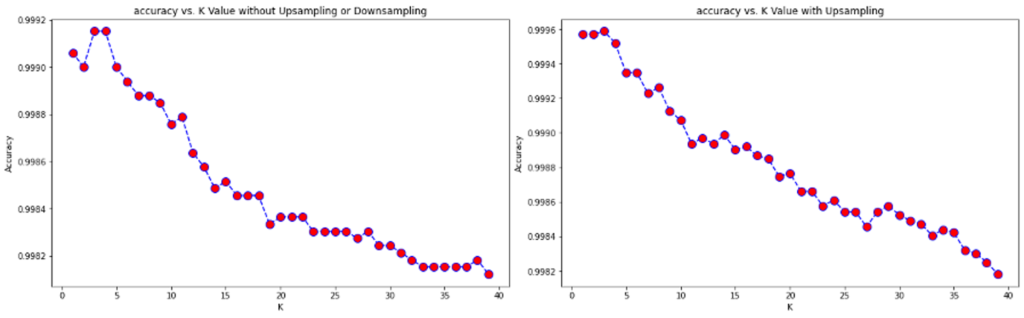
Here, the strong dependency of accuracy with respect to different numbers of neighbours is evaluated. Number of neighbors with k = 3 shows the highest accuracy in this case. However, the distribution of training data between the background and shadows present in the image is not balanced. There is little information about shadows in the training data. Therefore, upsampling the smaller portion of the labeled data is necessary in this case. The results using upsampled training data is shown in figure 3 on the right side. The accuracy increases slightly with the number of neighbors with this method. Hence, the final model was applied with the upsampling method, while k was chosen to be three.

Next, the size of the input image has an impact on the computation time required. Therefore, the influence of image size on mean squared error (MSE) and computation time were also evaluated. In figure 4, it can be seen that the images were resized from 2048 × 2048 to 1024 × 1024 (1/4), 512 × 512 (1/16), and 256 ×256 (1/64).

 

 

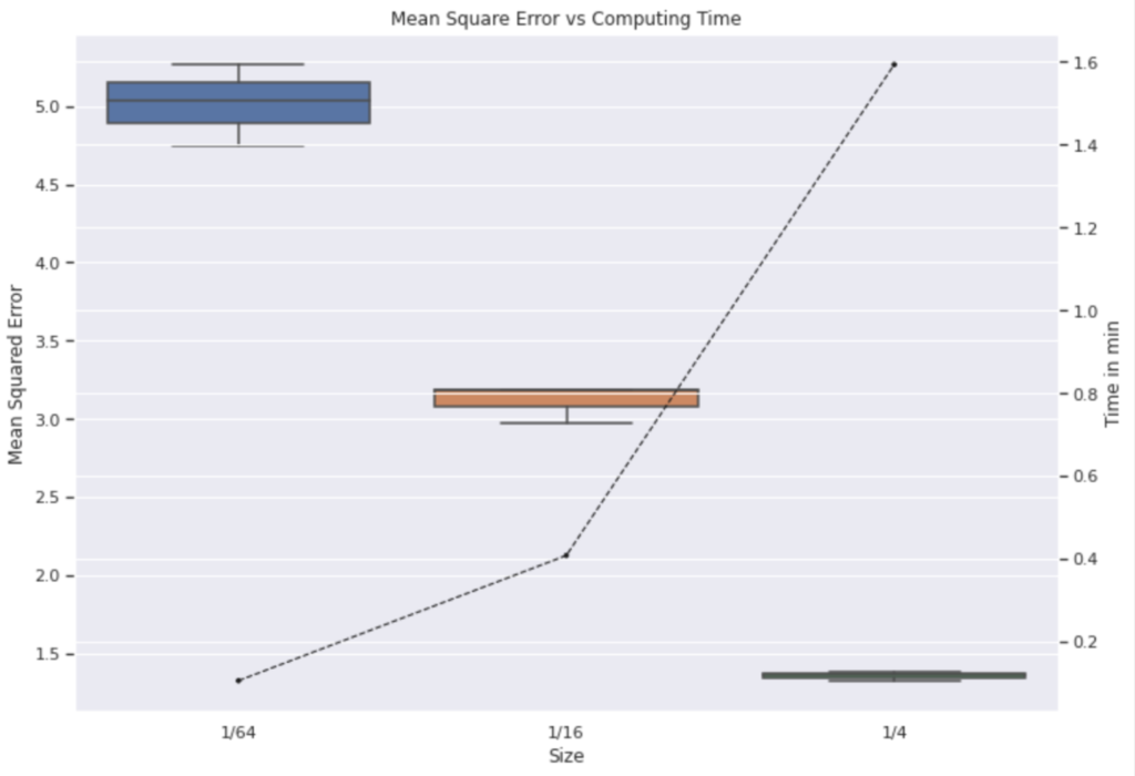
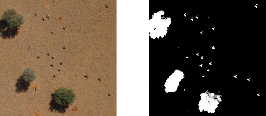
Resize means in this case that the pixel information will be changed. Smaller sized images contain few pixels and larger size images which contain more pixels. This results in a lower computation time for smaller images, while however increasing the predictions Mean Square Error. Moreover, it is interesting that the smallest images have a wide variance of MSE and the graph of computation time (dash line) shows non-linear behaviour. Therefore, images were resized with ratio 1/16 as a trade off between MSE and computation time. At the end, the output of this algorithm is a binary image as shown in figure 5 on the right side.

 

 

Shadow Detection Process

Now, the binary image, in which the pixels classified as shadows are assigned the color white (0) and other pixels are assigned the color black (1), is subjected to an image transformation pipeline to identify and extract individual shadow regions. These extracted regions containing shadows of different objects such as trees, bushes and animals are used to train the image classification model. The package opencv [1] is used to conduct the following steps. 1. Preprocessing by morphological transformation 2. Contour detection and analysis 3. Cropping out the shadows from the binary mask and the original rgb-image

Preprocessing by morphological transformation

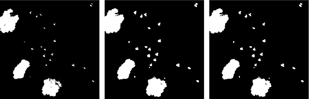
There are two basic morphological operations: erosion and dilation. Both operations are applied to a particular area called kernel, sliding over the binary image (similar to 2D convolution). When applying erosion, all pixels in the selected area are set to 0, if at least one pixel in the area is 0. Therefore, white areas, smaller than the kernel size (like white noise), are erased and falsely connected objects are detached from each other. Dilation works exactly the other way around. If at least one pixel in the kernel is 1, all pixels are set to 1. Consequently, if dilation is applied after erosion, the object’s white space that was reduced by erosion for noise reduction is now enlarged again. Also, broken up objects are re-connected.

For the example image, we used a 2-step approach with the following kernels:

• Dialation with a 15×15 kernel
• Erosion with a 3×3 kernel

In Fig. 5, you can see the evolution from a binary mask through all steps of the morphological transformation.

 

 

Contour detection and analysis

Contours can be defined as a curve joining all continuous points along the boundary of an area with a constant color value. Contours are useful for object detection and shape recognition. For contour detection in the morphologically transformed mask, we used the opencv function findContours with external retrieval mode and simple chain approximation. The external retrieval mode “retrieves only the extreme outer contours[2].” Therefore, smaller contours enclosed within a larger contour are disregarded. The simple chain approximation of the findContours function condenses the continuous curve into just the end-points that are representative of the shape of the contour. This helps in saving memory and reduces the number of data points generated for each contour. “For example, an up-right rectangular contour is encoded with four points[3].”

After contour detection, contours falling outside a specified size range were filtered out, as too small contours are usually grass shadows that are not of interest, and too large contours are areas outside the image slice.

As a result, a dataframe with the following contour information is created. All x, y coordinates are given for the top left corner of the respective area: * name * gps coordinates of the contour bounding box * x, y of the binary mask slice in the original ortho * x, y of the contour bounding box in the binary mask * width and height of the contour bounding box * contour perimeter * contour area * contour centroid * location of a fitted line through the contour * length of the fitted line

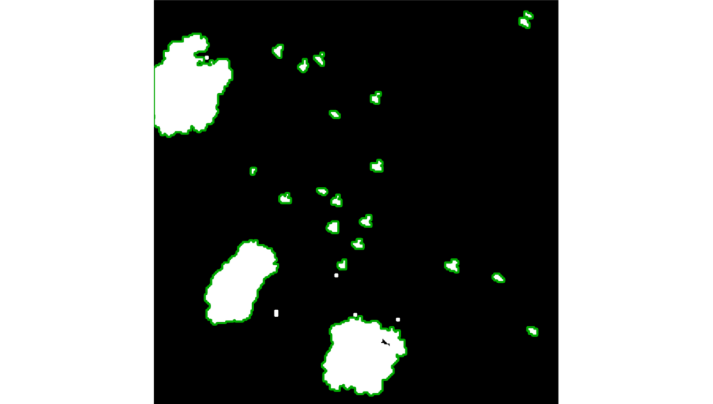
Fig. 6 shows the found contours in green in the morphologically transformed image.

 

 

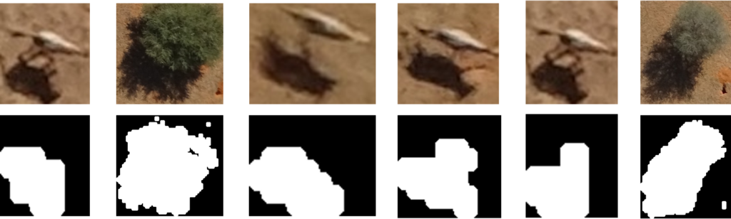
Cropping out the shadows from the binary mask and the original rgb-image

Afterwards, the bounding boxes of the contours are cut out of the binary mask and the original rgb-image. Examples are shown in Fig. 7. The RGB-cutouts are then used as training data for an image classification model.

 

 

Dataset Creation

To prepare the cutouts as inputs to a neural network, three more steps in the following orders were performed:

• Manuel labeling of objects (either animals, trees or bushes)
• train-test split
• data augmentation of the train data

Following some criteria, the cropped out images were identified as either animals, trees or bushes manually. This created the labels of the cutouts in order to perform a supervised learning classification task.

The whole annotated cutouts were randomly divided into train and test data in the ratio 90:10. Ninety percent of the cutouts, defined as the training data, went under data augmentation before being fed into a neural network.

Data Augmentation

Data augmentation is a technique to increase the diversity and amount of the existing data by applying random transformations to it. Examples of transformations include rotation (flipping the image up-down or left-right), cropping as well as adjusting brightness, contrast, saturation and hue of an rgb image. Figure 8 shows an example of how data augmentation randomly transforms a cropped out animal image in the training set. By gaining slightly modified copies of the existing data, data augmentation increases the amount of training data and thus helps to reduce possible overfitting.

 

 

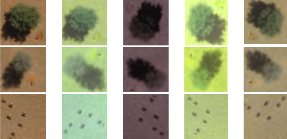
With our settings, our final training set was expanded to six times the original number of images. These images were then fed into a neural network for training. During model evaluation, we identified 3% better training accuracy with the augmented training set compared to the original set.

Model Selection and Evaluation

To decide which network fits best to our case, we started to evaluate the Sequential model from Keras Tensorflow first [4]. A set of functions were defined within the training module of these models that would enable the reconfiguration of neural network layers like 2D convolution or max pooling.

model = Sequential([
    data_augmentation,
    layers.experimental.preprocessing.Rescaling(1./255),
    layers.Conv2D(16, 3, padding='same', activation='relu'),
    layers.MaxPooling2D(), . . .)

When testing a small data set, quite high prediction probabilities were already achieved here with the validation data set containing random images. On closer inspection, however, it was found that the validation accuracy here only reached a value of about 80% and the model tended to overfit. Therefore, we decided to investigate further models and to optimize and evaluate them with respect to different neural networks and optimizers based on performance rankings. Based on the relevant literature and the size of the networks, we decided to investigate the neural networks DenseNet121 and MobileNetV2 as well as the optimizers Adam and Stochastic Gradient Descent (SGD). This results in four combinations, which offer different parameters that can be adjusted. Among these, we have chosen the ones that have the greatest impact on our accuracy.

For example, the following graphs show the validation accuracy of MobileNetV2 with an Adam Optimizer and DenseNet121 with SGD. For MobileNetV2, in addition to the batch size and the number of epochs, the learning rate, an alpha parameter describing the different filters and the input shape of the images in the three image color channels were examined. After several parameter tests, a batch size of 16, a learning rate of 0.0001, an input shape of (512,512,3) and an alpha value of 0.5 have been proven to be the best values. The corresponding graph can be seen in Fig.9 on the left side. Thereby it can be noted that the alpha value has only a very small influence on the performance of the neural network and that a lot of epochs are needed to achieve a higher level of validation accuracy after a constant phase in the first 150 epochs. A large number of epochs and large input shapes lead to increased computation time compared to other approaches.

 

 

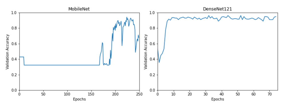
Another Convolutional Neural Network (CNN) architecture with a small model size (33 MB) and good performance is provided by DenseNet121. For hyperparameter tuning, the optimizers offer more parameters to vary and for the model three different pooling modes can be chosen. As a first step, the learning rate is being refined, different batch sizes are used and the number of epochs are varied. By comparing the different training runs acceptable parameters could be found. As a final step, the different pooling modes (average, max pooling and no pooling ) are applied on the training data set.

The Key-Performance-Indicator for the comparison is mainly the validation accuracy, where a maximum value of 96,1% could be achieved as it can be seen on the right graph of Fig. 9. It’s evident that the second variant provides better performance, since higher validation accuracies are achieved over a more constant time period. As a second indicator the difference of the loss and validation loss is considered, where values close to zero define a good performance. The maximum of the validation accuracy is obtained by using the Adam optimizer with a learning rate of 1E-05 and an epsilon of 1E-07. The DenseNet121 model is applied with no pooling and the default input shape of (224, 224, 3).

These parameters of the model DenseNet121 and the optimizer Adam are then used for training on the augmented data set. The found weights are saved and used for the validation data set to predict the different classes [tree, bush, animal]. The predicted labels and the respective confidence scores are added to a final data frame.

Project Result

As a result of our project, a data frame has been created with information about the shadow contours such as the area, the bounding box, the projected tree height, the predicted label and the confidence score. This was achieved by integrating different modules: Starting with the KNN approach to create binary images that contain different shadow objects, a contour extraction method was developed and the shadows could be detected and classified.

Figure 10 below shows an example of how the knowledge gained so far was used to generate a visualization of the data. The different areas were highlighted in color and the detected areas were marked with the corresponding labels.

 

 

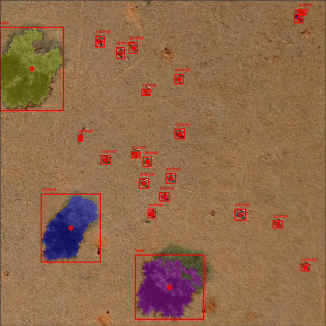
In order to locate the different objects predicted by the classification model on the original geoTIFF image (the raw image captured by the UAVs that contain the geo-referencing information), a small circle was drawn around the centroid of each of the bounding boxes. The outcome of our project aims to support wildlife conservation work in the Kuzikus Wildlife Reserve by detecting and classifying shadows. Although a high validation accuracy could be achieved, the developed classification model still needs improvement, because single wrong classification of shadows can occur. To solve this problem, the long-term goals should be to further optimize the model and to use a larger data set.

Conclusion

By developing a machine learning algorithm, our shadow detection team of Wild Intelligence Lab and TechLabs Aachen developed a tool to make a lasting contribution to automated data collection for ecosystem conservation in the Kuzikus wildlife reserve in Namibia. By extracting information from the contours of the shadows, a method for characterizing the ecosystem is created without disturbing the natural balance. In this way, the natural habitats of different breeds can be determined, or conclusions about the fertility of the land can be drawn from the accumulation of particular tree species in an area. By combining innovative technologies with machine learning and already gathered experience from previous projects of the locally acting Kuzikus team, important data for the protection of an ecosystem can be obtained.

 

 

For further information and upcoming achievements in wildlife conservation, please refer to the following links. Thanks for reading and taking part in nature preservation! Stay tuned!